Prototyping a Dipole Bass System
This article is the third and final installment in the series on my 4-way open-baffle loudspeaker prototype. In Part 1, I described the principles of open-baffle speakers and set up the first prototype using the miniDSP 2×4. Then, in Part 2, I used more sophisticated measurement techniques to set up the crossovers and equalization, and included a pair of sealed subwoofers to provide the lowest frequencies.
For this article, I aimed to replace the sealed subwoofers with open-baffle, or “dipole,” subwoofers. Although it’s possible to find a lot of material on placement of boxed subwoofers, there is not very much specific to dipole subwoofer placement. I realized that I needed to understand the bass behaviour of my room better, with respect to both monopole and dipole subwoofers, and so embarked on a series of measurements. The results of this investigation also form part of my baseline for acoustic treatments, as per the Bass Integration Guide – Part 1.
A little room mode theory
The theory item for this article is room modes – resonances or acoustic standing waves that are set up between the boundaries of the room. While there is more to room acoustics and the interaction of speakers with a room than just the modes, at subwoofer frequencies the room modes dominate, so I will focus on those for this article.
Basic of room modes
Let’s explore the concept of room modes with the aid of Figure 1. Assume that the left-most line represents the left wall, and the right-most line the right wall. The numbers along the bottom of each plot represent the distance across the room in percent: zero percent, 25%, 50%, 75%, and 100%. The vertical scale represents the magnitude of the standing wave, and thus the sound pressure level.
The first-order mode is the lowest frequency standing wave that the room can support. From the figure, you can see that the sound pressure will be high at the walls, and zero in the middle of the room. The second-order mode, at twice the frequency of the first-order mode, has high sound pressure at the walls and in the middle of the room, and zero sound pressure at the 25% and 75% marks.
The high-pressure areas are called anti-nodes, and the low-pressure points are called nodes. As the order of the mode increases, the number of nodes and anti-nodes between the two walls increases accordingly. Although the figure shows the first four modes, there are many more.
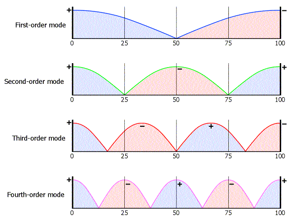
Figure 1. Illustration of room modes in one dimension
Modes such as those we have just discussed occur in one dimension, between two opposing walls, and are called axial modes. There are similar axial modes along the length of the room, and in the vertical direction between floor and ceiling. In addition, there are modes that occur between the four walls, and between any opposite pair of walls and the floor and ceiling – the tangential modes. Finally, there are modes that occur between all six room boundaries – the oblique modes. Consider also that there are many more than the four lowest-order modes indicated in the diagram, and you can see that the modes in a room quickly become too complex to calculate by hand.
Fortunately, there are a number of online mode calculators; one I like is Dr. Jörg Hunecke’s Room Eigenmodes Calculator. (This is a Java applet; if you have trouble running it in your browser, first check that you have Java installed and enabled, and if it still doesn’t work, try another browser. On my Mac, I found Chrome problematic but Safari worked fine.) Figure 2 shows the results of entering my key room dimensions into the Hunecke mode calculator. It lists the first twenty modes, which in my room run up to just under 90 Hz. (I have marked the approximate location of my left and right speakers L and R, and the listening position as X.)
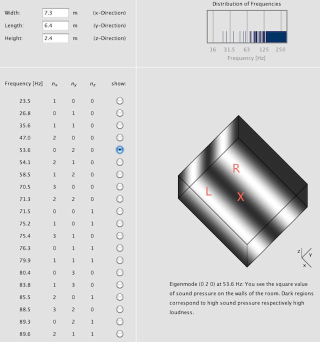
Figure 2. Hunecke room mode visualization
To identify a mode, the notation (x y z) is used. Each number is the order of the mode along the room length, width, and height respectively. (If you notice that I have the length and width swapped in the screenshot above, it is so that I can use the normal convention where the longest dimension is the first number.) The axial mode (1 0 0) is the lowest frequency resonance that occurs along the length of the room – in my case, this occurs at 23.5 Hz. This is sometimes referred to as the “fundamental frequency” of the room.
The next mode is (0 1 0) at 27 Hz, which is the first order mode across the width of my room. Then (1 1 0) at 36 Hz, the first tangential mode between the four walls. And so on. As the frequency increases, the modes become more numerous. The frequency at which the modes become so numerous that the room is no longer considered to act as a set of discrete modes is called the Schroeder frequency, which in my room occurs at a calculated 146 Hz.
Monopole subwoofers and room modes
When a monopole subwoofer – one that radiates equally in all directions – is placed in an anti-node (high pressure point) of a mode, it will excite that mode strongly. Elsewhere in the room, a microphone placed at an anti-node will tend to show a peak in the response at that frequency, and a microphone placed at a node will tend to show a null (dip). The corners of the room are anti-nodes for every single mode, so a subwoofer placed in a corner will tend to excite all room modes. This will result in the highest bass levels, but will also mean that the measured frequency response in the room is likely to be quite “peaky.”
If a subwoofer is placed at a node (low-pressure point), however, it will tend to not excite that mode. Referring to Figure 1, placing a subwoofer at the 50% location will tend not to excite the first and third-order modes; it will, however, excite the second and fourth-order modes. There is no location in the room that is a node for all modes – wherever you place a sub, it will excite at least some of the modes.
More than one subwoofer can (in theory) be placed to cancel excitation of specific modes. Figure 1 shows the positive phase of each mode in red and the negative phase in blue. Placing a subwoofer on the left wall and another on the right wall will excite the first-order and third-order modes in opposite phase, for a net zero excitation. The second- and fourth-order modes will not, however, be cancelled. In general, the problem of optimizing multiple subwoofers for the best overall response is complex, and some research has been done on algorithmic optimization solutions, notably the paper by Welti and Devantier, Low-Frequency Optimization Using Multiple Subwoofers. There is also good information on this topic in Chapter 13 of Toole’s book, “Sound Reproduction: The Acoustics and Psychoacoustics of Loudspeakers and Rooms.”
Dipole subwoofers and room modes
While a monopole subwoofer will excite modes in any direction, a dipole is directional, so how will it interact with modes? If the dipole is aligned with the room axes, as shown in Figure 3a, then we would expect that it will excite modes only in direction y. If, however, it is positioned at an angle as in Figure 3b, then it will excite modes in both the x and y directions. Thus, for dipole subwoofers, alignment with one or other of the room axes seems desirable.
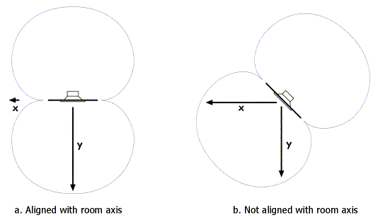
Figure 3. Dipole orientation
This cursory analysis is confirmed by John Kreskovsky in The truth about Cats and Dogs, and Mice; a story of dipole, cardioid and monopole woofers. Kreskovsky also identifies the key differences in the manner in which room modes are excited by monopoles, dipoles, and cardioids (the last being “out of scope” for this article). Because the front and rear waves of a dipole are out of phase with each other, the interaction with room modes along the dipole axis is different. Placing the dipole at a (pressure) anti-node will tend to not excite that mode; whereas placing the dipole at a node will tend to excite that node. This behavior is effectively the opposite of a monopole, and thus throws any conventional wisdom about subwoofer placement out of the window when dipole subwoofers are used.
Kreskovsky also points out that placing a subwoofer close to the listener is another technique that can be used to reduce the effect of room modes, by increasing the ratio of direct sound over that due to modes. Furthermore, in Dipole woofer on axis response in relation to listening distance, Kreskovsky shows that the 6 dB dipole rolloff applies only at an infinite listening distance; at shorter distances, the rolloff levels out at low frequencies. In the particular example given, a listening distance of 4 feet requires 8 dB less boost at 20 Hz than the commonly-assumed 6 dB/octave rolloff would indicate.
A dipole also has a different interaction with the rear wall, as explained in The Influence of Boundary Reinforcement on Monopole, Dipole and Cardioid Woofers. Specifically, a dipole woofer has a rolloff at low frequencies caused by the reflection off the wall behind it; and while not stated in the linked paper, the frequency at which the rollof begins will be higher the closer the woofer is to the wall. These points all indicate that the optimum location for a dipole subwoofer is likely to be a) aligned with a room axis, b) close to the listener, and c) as far away from the wall behind it as possible.
Investigative measurements: monopoles
To begin the study, I measured a number of responses with a sealed subwoofer. Candidate subwoofer locations are shown on the floorplan in Figure 4 as M, N, O, and so on, except for T, which for practical reasons can only be used as a microphone position.
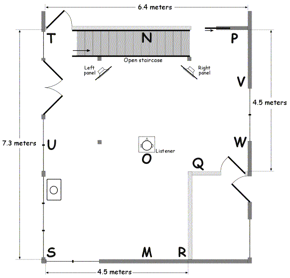
Figure 4. Floorplan of my listening room, showing candidate monopole subwoofer locations
Room characterization
To measure the response of the room itself, both the subwoofer and the microphone need to be placed in corners. The corners are anti-nodes for all modes, so placing the sub in a corner will excite all modes, and placing the microphone in a corner will pick up all modes. The purpose of this measurement is to confirm that the modes detectable in measurement correspond to the modes given by the mode calculator.
My house is a drywall on wood-frame construction on piers, and so is relatively lossy acoustically. This is actually a good thing, as the room modes are not as high a Q (“peaky”) as they would be in, say, a concrete bunker. It does, however, make it more difficult to illustrate the effects of the modes clearly.
I placed a sealed subwoofer in location P (on the floor), and the microphone in location T, also near the floor. The frequency measurement is shown in Figure 5, annotated with key modes. Comparing with Figure 2, the peaks on the frequency response plot generally correspond fairly well to axial modes identified by the mode calculator, with the clearly visible modes indicated on the figure. Some other modes that are not so clearly shown as peaks in the frequency response are also marked for completeness.
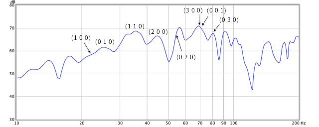
Figure 5. Room modes visible in a frequency response measurement
One point to note is that fundamental room mode (1 0 0) is not excited strongly at all. I suspect that this is because of the open stairwell at the front of the room, which prevents the mode building up pressure there. The region around 35 Hz is interesting, as there appears to be a very strong excitation of the first tangential mode (1 1 0). It is however worth noting that the 4.5m length along two of the walls has a first mode at 38 Hz, so there may be some effect in this area caused by the irregular shape of the room.
Listening position measurements
I moved the microphone to the listening position, and measured the response of a single sealed subwoofer placed in the locations shown in Figure 4. This was done with the thought that very low frequencies may be need to be generated by sealed subwoofers instead of dipole subwoofers – at this point, I had no idea whether dipole subwoofers would have adequate output at low frequencies.
Figure 6 illustrates in red the response of the corner subwoofer P, measured at the listening position. There are strong peaks observable at the length modes (2 0 0) and (3 0 0). In blue is the response of a subwoofer at location N, midway along the front wall – this is overall the best of the locations measured.
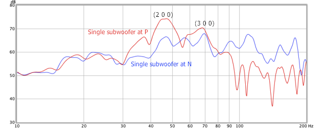
Figure 6. Frequency response of single monopole subwoofer
Visible in the plot for N is a notch centered around 80 Hz. This appears to varying degrees in many of the measurements below, and appears to be related to a cluster of odd-order modes in this area:
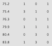
Problem mode cluster
Figure 7 shows the decay plot generated from the measurement at location N, with the 20 dB decay target shown as a black line. The room fundamental (1 0 0) at 23 Hz shows up more clearly in the decay plot than in the steady-state frequency response measurement, as does the first-order width mode (0 1 0) at 27 Hz. The slow decay time at the second and third-order modes between 40 and 80 Hz also looks rather less satisfactory than the simple frequency response plots alone might indicate. The decay plot appears to indicate some resonance in this room in the sub-20 Hz area, which I suspect may be due to the open stairway and the upstairs hallway to which it leads.
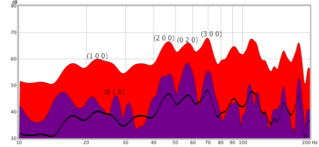
Figure 7. Decay plot of the best monopole sub, at location "N"
Of the other locations measured, location O, right behind the listening seat was – surprisingly – slightly worse than N in terms of response flatness, and comparable in terms of decay performance. Location R had good response up to 80 Hz, but poorer decay performance. The other locations – M, Q, S, U, V, W – all had significant peaks and dips, and poorer decay performance.
I also measured pairs of symmetrically-placed subs, at M+N, U+W, and the 25% locations into the room (near the main panels). The M+N pair performed the best of these, and had better decay performance than the single sub at N but with a dip in the frequency response at 56 Hz. I decided to not pursue this further at this point.
Investigative measurements: dipoles
I now needed to conduct a series of experiments to determine the effect of dipole subwoofer placement and orientation in my room. The candidate locations are shown in Figure 8 as A, B, C, and so on, along with the useful orientations of the dipole axis.
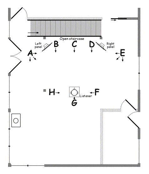
Figure 8. Floorplan showing candidate dipole subwoofer locations and orientation
Locations A through E are the “conventional” locations that I would likely have used if I were simply plonking panels down into the room without trying to use measurements to find the best location. Locations F and H are based on the “nearfield” idea: close to the listener to benefit from the shelving that occurs at close distances and low frequencies, and far away from the walls to minimize the effect of reflection of the rear wave. Location G is an experiment in placing the subwoofer very close to the listener.
In order to assist in interpreting the measurement results, I applied a “textbook” dipole rolloff compensation filter to the dipole subwoofers. Since a dipole subwoofer rolls off at 6 dB/octave, I applied a shelving filter that drops response by 12 dB between nominal corner frequencies of 30 Hz and 120 Hz i.e. two octaves. This covers the frequency range of interest for the dipole subwoofers, and allows the measurement results to be interpreted in a conventional manner – that is, with respect to a nominally flat reference.
Dipole subwoofer orientation
The first thing that I wanted to do was to confirm that orientation of a dipole subwoofer affects mode excitation. I placed a dipole subwoofer at A and the microphone at the listening position. Figure 9 shows the results with the dipole oriented along the length of the room in green, across the room in blue, and at 45 degrees in red. While there are some differences due to orientation, it is hard to identify that they are mode-related. The 45-degree orientation does generally have peaks wherever either of the other two traces have a peak.
In summary, while there are differences due to dipole orientation, they are hard to predict from the room modes, and are for the most part less significant than variations within any one curve.
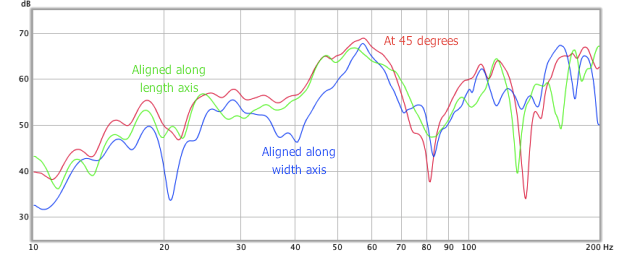
Figure 9. Effect of dipole orientation at listening position
Dipole subs in pairs
If dipole subs are placed in pairs in mirror-image locations in the room, and facing each other, how does the response differ? I had expected that the width modes would be excited differently. This does not, however, seem to be the case to any significant degree, at least in my listening room. In Figure 10, the response from a dipole subwoofer placed at A, and facing across the room, is shown in purple (the same plot as in Figure 9); with subwoofers at locations A and E, pointed towards each other, the response obtained is shown in blue. There are some changes, but the curves are essentially the same but with a higher level.
I then rotated the two subs to face along the length of the room. This curve is shown in Figure 10 in green. In this case, there is a distinct difference in the shapes of the curves, with the second-order length mode (2 0 0) being strongly excited, and the second-order width mode (0 2 0) less so.
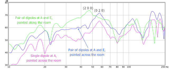
Figure 10. Effect of symmetric dipole pair
Nearfield dipole subs
Does placing a dipole sub “nearfield” to the listener provide any benefit? To test this, I placed a sub at H, and measured the response at the listening position. This measurement is shown in Figure 11 in purple. Shown on the same graph in blue is the response that was measured at A – clearly, the placement at H is a substantial improvement over A. Some of the difference may also be due to differing location along the length of the room, a factor I didn’t consider until after completing the measurements. So the answer is a qualified “yes.”
The response from a mirror-image pair of subwoofers placed at F and H is shown in Figure 11 in green. As before, the response is very similar to a single subwoofer but the magnitude is increased.
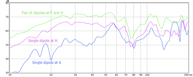
Figure 11. Effect of nearfield dipoles
Since the frequency response of the nearfield pair at F and H is quite good, I generated a decay plot, shown in Figure 12. Apart from the hole around 80 Hz, this is quite good for an untreated room, and falls a little short of the Guide’s target of 20 dB in 150 ms.
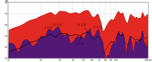
Figure 12. Decay plot of nearfield dipoles
Placing a dipole subwoofer too close to the listening position, however, can be detrimental. A subwoofer placed at G, right behind the listening seat, had a poor response, presumably because the subwoofer was on the floor and the listener’s ear (microphone position) was now getting close to the dipole null.
Asymmetric mode cancellation
If multiple dipole subwoofers are used at asymmetric locations in a room, can delay on one or the other be used to smooth the combined response? To test this, I placed a subwoofer at B, next to the left panel, and one at G, right behind the listening seat. Figure 13 shows the response of both subwoofers, with no delay between them, in red. I applied varying amounts of delay to each subwoofer. In blue is the flattest response obtained, with 5 ms of delay applied to the subwoofer at B. With more subwoofers, getting the optimum delay between them all could be quite challenging.
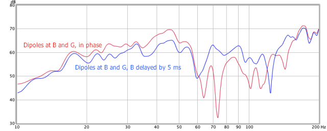
Figure 13. Effect of delay between asymmetric dipoles
Subwoofer choice and location
At this point, I felt that I was armed with enough information about how monopole and dipole subwoofers behave in my room to come up with a “go forward” plan. After a number of false starts and dead ends, though, I remembered the K.I.S.S. principle: Keep It Simple, Stupid! In the end, the best compromise between sound quality and practicality in my room consists of just a single dipole subwoofer.
An early realization was that flat panels are a poor choice for dipole subwoofers. I began with two prototype panels positioned at F and H, since these had by far the best measurements (Figure 11). At high levels, the panels moved enough to vibrate the floor – a disturbing effect, and not one I liked at all! I realized that opposing drivers in “push-pull” configuration would be needed, so I built a prototype sub using four Exodus Audio DPL-10 drivers in the configuration illustrated in Figure 14. This could be thought of as either a folded flat baffle or partway to a Linkwitz “W-frame” dipole subwoofer.
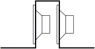
Figure 14. Folded baffle dipole subwoofer
The photograph below shows the construction of the prototype. While too flimsy for long-term use, it proved adequate for testing and measurement, and thus to prove the concept.
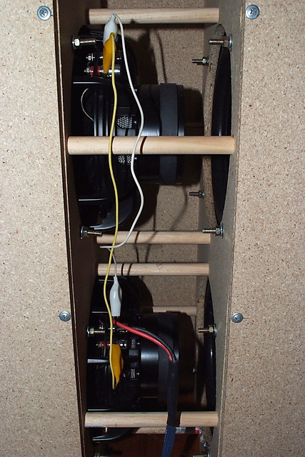
Prototype folded-baffle dipole subwoofer
I used two locations for this subwoofer, marked as F and Q in Figure 15. Location F in blue is acoustically the more optimum location, although it takes “some getting used to,” as a large panel within arms-length of the listening seat is visually quite distracting. Location Q is more practical in terms of room usage, but since one side of the baffle is blocked by the wall, we wouldn’t expect it to develop the full dipole radiation pattern. Also shown is location H in grey, a potential location for a second copy of this subwoofer, once a visually more acceptable design has been produced.
During the setup process, I also ran measurement sweeps in a constellation of locations around my nominal listening position. As a result, I moved the listening seat about 40 cm forward. The listening arrangement is now an equilateral triangle 2.4m on each side.
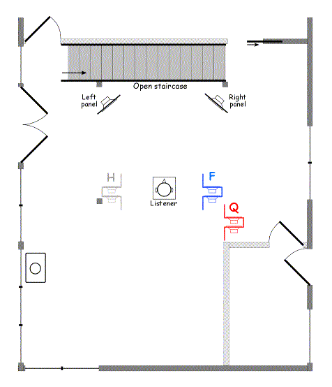
Figure 15. Revised listening room layout with dipole subwoofer locations
Figure 16 shows the measurements of location F in blue, and location Q in red. It is interesting to note that the peaks at around 53 and 70 Hz are at the same level, but that location F has around 5 dB more output below 45 Hz. While I was able to make both locations work, location F is clearly preferable in terms of higher output capability, and reduced excursion and thus distortion at low frequencies.
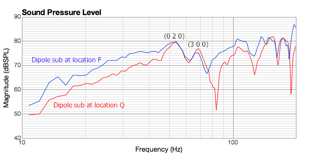
Figure 16. Response of dipole subwoofers at locations F and Q
Equalizing the response of the subwoofer at location F to flat, up to 125 Hz, was a fairly simple matter, requiring only a notch filter at 53 Hz and a second (probably not really necessary) one at 107 Hz. The resulting response is -3 dB down at around 30 Hz. That this 30 Hz performance was obtained with no dipole compensation boost supports Kreskovsky’s analysis with regard to dipole response as the distance to the listener decreases.
The crossover between the subwoofer and main panels took many trials. I found, during my many twists and turns, that I was at times able to detect the sound of steep highpass filters in this frequency range as a “phasy” or tunnel-like effect. I did not, however, want to use a shallow slope on the subwoofer, because of the risk of localizing the sub over to my right. I have, for now, settled on a (symmetrical) 24 dB/octave Butterworth crossover at 80 Hz. This is something that I intend to experiment with further.
The resulting in-room response is shown in blue in Figure 17. The notch in the 80 Hz area is still present, although not as severe as in some of the measurements above; it will be interesting to see if acoustic treatments are able to reduce the problems in this area.
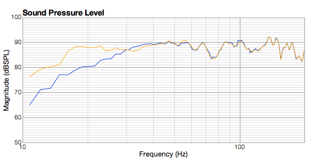
Figure 17. In-room response of integrated dipole subwoofer
While the 30 Hz rolloff is very good performance, I have long imagined in-room response to 20 Hz and below to be desirable, as signal theory states that the energy in a transient signal extends well below and above the nominal steady-state frequency response of an instrument’s notes. I did some quick analysis of a number of music samples using Audacity, which showed that very percussive, dynamic tracks do have significant energy between 20 and 30 Hz, although well below the main energy peaks (typically 40 to 50 Hz for bass guitar, and 60 to 80 Hz for drums).
I found that it was not too difficult to extend the response down to 20 Hz, either by equalizing the dipole subwoofer with a shelving boost, or by adding in a sealed subwoofer low-pass filtered around 30 Hz. Figure 17 shows the measured result of the latter in orange. Listening to this configuration, however, gave a resoundingly neutral score in its favour! On many tracks, it was hard to tell the difference. On others, there seemed initially to be an increased sense of space, but a series of A-B switches put in doubt this initial impression. At times, I felt that the sound became muddier. I eventually ran a decay plot and realised that I was perhaps noticing low-frequency resonances excited by the monopole subwoofer – the same ones visible in Figure 7.
This exercise left me wondering what benefit a “flat to 20 Hz” response really has. For acoustic recordings (outdoors or in large venues), it is conceivable that there are environmental sounds in the recording that add to the realism of reproduction. For studio recordings, one wonders how many studio monitors themselves reproduce down to 20 Hz accurately. Perhaps this would be a good topic to explore in a future article.
At any rate, I am for now sticking with the single uncompensated dipole at location F. With approximately 200 Watts of power available per driver, listening at higher volumes showed that this single sub provides more than adequate output for any reasonable listening level. Nonetheless, once I have come up with a visually more appealing design, I plan to add a second subwoofer at location H. At that time, I may again experiment with a shelving filter to boost those very low frequencies.
Analysis
The decay plot of the integrated subwoofer and woofer (one channel only – in this case the right channel) is shown in Figure 18. The 20 dB target is shown as a black line. This is good for an untreated room, but there are distinct resonances visible above 45 Hz that should be addressed by acoustic treatment as per the Bass Integration Guide – Part 2.
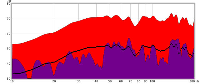
Figure 18. Decay plot of integrated dipole subwoofer
The waterfall plot, in Figure 19, shows the resonances in a different view. For comparison, Figure 20 shows the waterfall plot of the system with the dipole subwoofer positioned at location Q. As would be expected from Figure 16, more equalization was needed at this location. The waterfall also shows that this location suffers more from room resonances than location F. Whether this holds true after acoustic treatment remains to be seen!
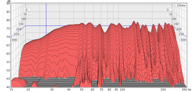
Figure 19. Waterfall plot of integrated dipole subwoofer at location F
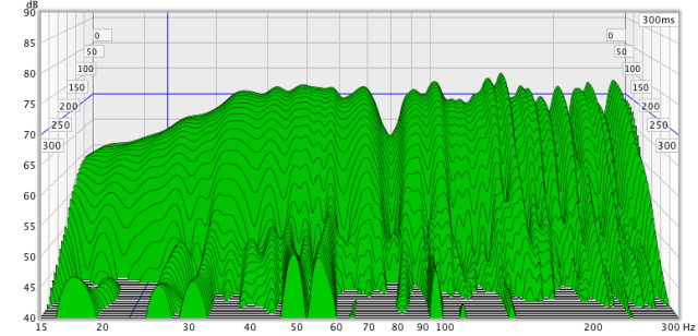
Figure 20. Waterfall plot of integrated dipole subwoofer at location Q
One final note. The Bass Integration Guide suggests that a “target curve” be applied to the end result. Although it is recommended after acoustic treatment, I decided to experiment with it at this point anyway. Up until now, I had been using equalization on each output channel of the miniDSP to adjust the response of each driver. For overall frequency response tailoring, however, equalization on the input channels should be used. A low-shelf boost is easily used to shelve up bass frequencies and provide additional solidity and oomph on the bottom end.
Concluding remarks
This concludes the series of articles on the four-way open-baffle loudspeaker. I’ve learnt a great deal along the way, and have become very much a believer in using simulations, prototypes, and measurement. The prototype baffles – for both the main panels and the subwoofer – have served their purpose: to be an inexpensive learning tool and to enable me to measure and understand the behaviour of these drivers in this type of baffle.
It has been interesting to see how far such a cheaply-constructed prototype can be taken – much further than I had ever expected, in fact. At this point, the speaker does sound very good, with good imaging and reasonable dynamics and slam. The bass is tight and articulate, despite the flimsy baffle construction.
There are some issues that I haven’t been able to address, and which will be the subject of further work. Acoustic damping has already been mentioned, and a more solid set of baffles is also an obvious target. But, I would also like to explore other midrange and tweeter drivers. What is the saying… a DIY’ers work is never done? Perhaps one day I will be able to write an article on the completed speaker! In the meantime, happy open-baffling to you all.
Acknowledgments
This article was improved with comments from John Kreskovsky (Music and Design), Nyal Mellor (Acoustic Frontiers), and Paul Spencer. Nigel Addison provided an invaluable second pair of ears to help evaluate the speaker and keep me on track.
Some of the measurements in this article were performed with FuzzMeasure Pro, provided by Chris Liscio to HifiZine for the purpose of assisting with writing educational articles. Thank you for your support!


I recall an article from the ?’80’s? in an old UK magazine called Hi Fi for Pleasure, which described a full range dipole in development by Warfdale. Now memory does not serve well and may have been one of their April 1st articles unfortunately, but it described, I think, a dipole with HF on axis with the listening position ( say 60 degrees from back parallel to back wall), mid range at 45 degrees to back wall and bass at 30 degrees. Now numbers are based on again dodgy memory, but interestingly this was also speakers backing on to long wall, rather than the traditional short wall. Not sure how manouverable your subs are but assuming that my memory is not playing tricks ( I have never been able to find the original article or any evidence that it existed on the net in the last 10 years!) and it was not an April fools article, maybe moving them to postitions B and D and at 30 degrees to the back wall might be interesting?
I will eventually be trying this but am potentially another 3 to 5 years away from a room big enough.
Regards
Grant
Hi Grant, thanks for the comment! I did find a vintage Wharfedale open-baffle speaker on Troels Gravesen’s site: http://www.troelsgravesen.dk/vintage.htm, although not of the configuration you described. There is some discussion on John Kreskovsky’s site on rotating a dipole woofer for matching power response to on-axis sresponse: http://musicanddesign.com/PowerMatching.html
Very nice discussion/explanation regarding dipole subs.
Hi There
I am searching for a way to calculate the w frame dipole but find not much, I want to try a 2 x 18 inch subwoofer with this and shelfing, now I have a acoustical resistance box who go low but sound not fine.
Nice discussion.
regards
Kees:
Did you find anything on modelling/doing calculations for a W-Frame dipole sub? I want to build
something using some nice 10″ woofers, but don’t have a clue where to start the calculations.
Hi guys, Martin King has a worksheet for an H-frame dipole, it may be worth trying that using the same frame depth as your planned W-frame.
http://www.quarter-wave.com/Back_Door/MathCad_Models.html